Project 3
STATS 220 Semester One, 2026
Austin Sarney
Introduction
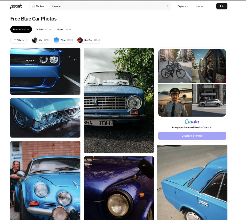
I used the words “blue car” because I started this assignment on a bus and the first thing I saw looking out the window was a blue car (I’m so creative).
https://www.pexels.com/search/blue%20car/

The 3 things I noticed about the photos were:
The majority of photos seemed to be of older cars instead of more modern cars which are more common to see in person.
There seemed to be a roughly equal proportion of portrait and landscape photos.
Most of the photos that I looked into had between 0 and 10 hearts, where 0 was the most common number of hearts that I saw.
My selected photos:
Key features of my selected photos
percent_blue <- mean(selected_photos$main_colour == "blue") %>%
  round(digits=3) * 100
90.9% of the photos I selected had more blue than red or green.
proportion_blue_portrait <- selected_photos %>%
  group_by(is_portrait) %>%
  summarise(proportion_blue = mean(main_colour == "blue"))

proportion_blue_not_portrait <- proportion_blue_portrait$proportion_blue[1]
percent_blue_not_portrait <- round(proportion_blue_not_portrait, digits=3) * 100
86.7% of the selected non-portrait photos have more blue than red or green.
mean_num_author_words_by_is_portrait <- selected_photos %>%
  group_by(is_portrait) %>%
  summarise(mean_words_in_author = mean(words_in_photographers_username))

non_portrait_mean_words <- mean_num_author_words_by_is_portrait$mean_words_in_author[1]

difference <- round(mean_num_author_words_by_is_portrait$mean_words_in_author[1] - mean_num_author_words_by_is_portrait$mean_words_in_author[2], digits=3)
Of the non-portrait photos, the average photographer username had 2 words.
In the selected photos, the usernames of the photographer had 0.429 fewer words on average if the photo was portrait.
Creativity

My project demonstrates creativity because I used the value of one of the extra variables I created in selected_photos inside an ifelse() function to have text for each image inside of my animated gif that dynamically changes the contents of the words that are added by image_annotate. This means that my gif can be somewhat informative about each image.
Learning reflection
I think an important idea from module 3 is that we can create more variables without needing to collect more data. Having TRUE/FALSE summary values are easier to work with for ifelse functions, and having them be part of the data frame means that I didn’t have to constantly rewrite the same line over and over comparing values from other columns.
I am curious about exploring more of how we can use APIs to automatically get data from frequently updating sources like weather forecasts to create dynamic reports which show us exactly the variables we care about by customizing the way we present the data once we have recieved it from the computer-readable JSON API.
Appendix
library(tidyverse)
library(httr)
library(magick)
library(stringr)

api_key <- Sys.getenv("apikey") #so I can upload this to github

url <- "https://api.pexels.com/v1/search?query=blue%20cars&per_page=80"

response <- httr::GET(url,
                      add_headers(Authorization = api_key))

data <- httr::content(response,
                      as = "parsed",
                      type = "application/json")

photo_data <- tibble(photos = data$photos) %>%
  unnest_wider(photos) %>%
  unnest_wider(src)

selected_photos <- photo_data %>%
  filter(str_to_lower(substr(alt, 1, 1)) == "a") %>%
  #Filter it down to only photos where the alt text either starts with "A" or "a".
  #This is personally relevant to me because A is the first letter of my name.
  mutate(
    is_portrait = width < height, #If the photo is a square then it isn't portrait, so this will be false
    words_in_photographers_username = str_count(photographer, "\\S+"),
    main_colour = ifelse( #If the red value is greater than the blue and green value
        strtoi(
          substr(avg_color, 2, 3), #Get the 2 hexadecimal digits after the "#"
          base=16
          ) > strtoi(
            substr(avg_color, 4, 5),
            base=16
          ) & strtoi(
            substr(avg_color, 2, 3),
            base=16
          ) > strtoi(
            substr(avg_color, 6, 7),
            base=16
          ),
        "red",
        ifelse( #yay nested ifelse :)
          #If the green value is greater than the red and blue
          strtoi(
            substr(avg_color, 4, 5),
            base=16
          ) > strtoi(
            substr(avg_color, 2, 3),
            base=16
          ) & strtoi(
            substr(avg_color, 4, 5),
            base=16
          ) > strtoi(
            substr(avg_color, 6, 7),
            base=16
          ),
          "green",
          "blue"
          #If any of the values are equal it will end up as blue
          #I don't think this is a problem with the data I selected
        )

    )

  )

write_csv(selected_photos, "selected_photos.csv")


# part D

percent_blue <- mean(selected_photos$main_colour == "blue") %>% #proportion of photos where the main colour is blue
  round(digits=3) * 100 #turned into a %
print(paste0(percent_blue, "% of the selected photos have more blue than red or green"))


proportion_blue_portrait <- selected_photos %>%
  group_by(is_portrait) %>%
  summarise(proportion_blue = mean(main_colour == "blue"))

proportion_blue_not_portrait <- proportion_blue_portrait$proportion_blue[1]
#proportion of the photos that are not portrait, which are mostly blue


mean_num_author_words_by_is_portrait <- selected_photos %>%
  group_by(is_portrait) %>%
  summarise(mean_words_in_author = mean(words_in_photographers_username))

difference <- round(mean_num_author_words_by_is_portrait$mean_words_in_author[1] - mean_num_author_words_by_is_portrait$mean_words_in_author[2], digits=3)
#mean_words_in_author for non portrait minus for portrait


# part E


images <- NULL
for (i in 1:nrow(selected_photos)) {
  current_image <- image_read(selected_photos$small[i]) %>%
    image_scale("300") %>%
    image_annotate(
      text = ifelse(selected_photos$main_colour[i] == "blue",
                    "BLUE PICTURE",
                    "NOT MOSTLY\nBLUE!!"),
      size = 35,
      boxcolor = "#FFFFFF",
      gravity = "north"
    )
  if (is.null(images)) {
    images <- c(current_image)
  } else {
    images <- c(images, current_image)
  }
}

image_animate(images, fps=1) %>%
  image_write("creativity.gif")
---
title: "Project 3"
author: "Austin Sarney"
output:
html_document:
code_folding: hide
subtitle: "STATS 220 Semester One, 2026"
---
```{css echo=FALSE}
@import url('https://fonts.googleapis.com/css2?family=Cal+Sans&family=Micro+5&display=swap');
.author, .title, .subtitle, h2 {
background: linear-gradient(90deg,rgba(131, 58, 180, 1) 0%, rgba(252, 69, 124, 1) 100%);
background-clip: text;
color: rgba(0,0,0,0);
background-size: 100% 100%;
background-repeat: no-repeat;
display: block;
width: max-content;
margin: 0px 0px 10px 0px;
}
.title {
font-size: 50px;
text-shadow:
0 2px 6px rgba(252,69,124,0.25),
0 6px 18px rgba(131,58,180,0.18);
} /* Its kinda subtle */
body {background: #EEEEEE;}
.author {font-family: "Micro 5", sans-serif;display: block;
width: max-content;}
h1, h2, h3 {font-family: "Cal Sans", sans-serif;display: block;}
div.section:not(#my-selected-photos, #the-3-things-i-noticed-about-the-photos-were), div#header {
background: rgba(255, 255, 255, 0.8);
border-radius: 10px;
padding: 20px;
margin: 20px;
box-shadow: 8px 7px 7px #AAA
}
.figcaption {
color: #777;
}
/* Fun fact: I started the CSS for this before I started revising for the test */
```
```{r setup, include=FALSE}
knitr::opts_chunk$set(echo=TRUE, message=FALSE, warning=FALSE, error=FALSE)
library(tidyverse)
selected_photos <- read_csv("selected_photos.csv")
```
## Introduction
I used the words "blue car" because I started this assignment on a bus and the first thing I saw looking out the window was a blue car (I'm so creative).
[https://www.pexels.com/search/blue%20car/](https://www.pexels.com/search/blue%20car/)
### The 3 things I noticed about the photos were:
* The majority of photos seemed to be of older cars instead of more modern cars which are more common to see in person.
* There seemed to be a roughly equal proportion of portrait and landscape photos.
* Most of the photos that I looked into had between 0 and 10 hearts, where 0 was the most common number of hearts that I saw.
### My selected photos:
`r selected_photos %>% select(url) %>% knitr::kable()`
## Key features of my selected photos
```{r, eval=TRUE}
percent_blue <- mean(selected_photos$main_colour == "blue") %>%
round(digits=3) * 100
```
**`r percent_blue`%** of the photos I selected had more blue than red or green.
```{r, eval=TRUE}
proportion_blue_portrait <- selected_photos %>%
group_by(is_portrait) %>%
summarise(proportion_blue = mean(main_colour == "blue"))
proportion_blue_not_portrait <- proportion_blue_portrait$proportion_blue[1]
percent_blue_not_portrait <- round(proportion_blue_not_portrait, digits=3) * 100
```
**`r percent_blue_not_portrait`%** of the selected non-portrait photos have more blue than red or green.
```{r, eval=TRUE}
mean_num_author_words_by_is_portrait <- selected_photos %>%
group_by(is_portrait) %>%
summarise(mean_words_in_author = mean(words_in_photographers_username))
non_portrait_mean_words <- mean_num_author_words_by_is_portrait$mean_words_in_author[1]
difference <- round(mean_num_author_words_by_is_portrait$mean_words_in_author[1] - mean_num_author_words_by_is_portrait$mean_words_in_author[2], digits=3)
```
Of the non-portrait photos, the average photographer username had **`r non_portrait_mean_words`** words.
In the selected photos, the usernames of the photographer had **`r difference`** fewer words on average if the photo was portrait.
## Creativity
My project demonstrates creativity because I used the value of one of the extra variables I created in selected_photos inside an ifelse() function to have text for each image inside of my animated gif that dynamically changes the contents of the words that are added by image_annotate. This means that my gif can be somewhat informative about each image.
## Learning reflection
I think an important idea from module 3 is that we can create more variables without needing to collect more data. Having TRUE/FALSE summary values are easier to work with for ifelse functions, and having them be part of the data frame means that I didn't have to constantly rewrite the same line over and over comparing values from other columns.
I am curious about exploring more of how we can use APIs to automatically get data from frequently updating sources like weather forecasts to create dynamic reports which show us exactly the variables we care about by customizing the way we present the data once we have recieved it from the computer-readable JSON API.
## Appendix
```{r file='exploration.R', eval=FALSE, echo=TRUE}
```
```{r file='project3_report.Rmd', eval=FALSE, echo=TRUE}
```